Amine M'Charrak

Tutorial: Monte Carlo Method for approximation of integrals

We will calculate the following integral:

1. Let us solve this integral analytically using our calculus knowledge from high school:

Integrating $sin(x)$ over $x$ gives us $-cos(x)$. Thus, we have

Great, so now that we let us use the Monte Carlo method to compute this integral numerically using Python!

1. First we will load the necessary python math packages.

%matplotlib inline
import numpy as np
from scipy import random
import matplotlib.pyplot as plt

Now we need to define the integration limits:

a = 0;
b = np.pi;
limits = (a,b);

We also need an array full of random numbers in our interval $(a=0,b=\pi)$ at which we will evaluate the function $sin(x)$. We choose 2000 random values sampled from the uniform distribution between $a$ and $b$.

nSamples = 2000;
xrand = np.random.uniform(a,b,nSamples);

Now let us define the function we are integrating over such that we can query its value $sin(x)$ for specific $x$ values.

def int_func(x):
    return np.sin(x)

Now we evaluate the function for all $x$

evals = int_func(xrand);

Now we use the following fact for calculating the average of any function f denoted as $\langle f(x)\rangle$:

Now solving for the integral itself we get the basic method for approximating any integral

Finally, we can use the Law of large numbers to approximate the RHS by writing done $\langle f(x)\rangle$ as the average of $N$ random samples as follows

From the last equation above we can see, that we have to add up all the evaluations of our randomly sampled ${x_i}$. So lets do that!

sum_evals = sum(evals);

The last missing part is calculating the ‘length’ of our interval $(a,b)$ which is

len_interval = b-a;

approx_integral = len_interval*(1/nSamples)*sum_evals;

Let us print out the final result and see if we can get close to the true value of 2:

print("Our Monte Carlo method estimates the integral from 0 to pi for the function sin(x) to be: %.5f" % approx_integral)

Our Monte Carlo method estimates the integral from 0 to pi for the function sin(x) to be: 2.04778

Using this simple method we get fairly close to the true value of 2!

BUT unfortunately, every time we run this approximation, we get another value. In order to get a better idea of the true integral value, we will now plot the histogram of approximated integral values for a bunch of runs. We should see, that the histogram will have a peak around 2 and falls of to both sides. Let us see if this is the case!

First we combine the above steps used to evaluate the integral into a single function with the only inputs being:

1. Integral function
2. Integral limits
3. Number of samples used for approximation

def approx_integral(int_limits,nSample,int_function):
    (low_lim,upp_lim) = int_limits;

    xrand = np.random.uniform(low_lim,upp_lim,nSample);
    evals = int_function(xrand);
    sum_evals = sum(evals);
    len_interval = b-a;
    return len_interval*(1/nSamples)*sum_evals;

nIter = nSamples;
approximations = np.zeros((nIter,1));
# create buffer to save approximation of each run
for iter in range(nIter):
    approximation = approx_integral(limits,nSamples,int_func)
    approximations[iter] = approximation

Now let us plot the histogram to see where our peek for these 2000 approximations we ran lies!

plt.title("Histogram of integral %d approximations" % nIter);
plt.hist(approximations,bins=25,ec = "black");
plt.xlabel("Approximated value")
plt.ylabel("Count")

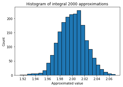
Finally, we see, that the histogram is centered around the approximated value of 2 and flattens out to both sides. We can reduce the uncertainty, i.e. variance of this histogram, by increasing the number of samples. When the number of samples approaches $\infty$ we should see an almost “delta-like” function with a peak at around 2!